Multivariate
pyreml takes one or several columns as response and performs multivariate analysis by modeling the covariance between them (e.g. Calus & Veerkamp, 2011; Jia & Jannink, 2012)
Formulation
For two responses \(1\) and \(2\) and two random effects \(\mathbf{a}\) and \(\mathbf{b}\), the model stacks response-wise:
\[ \begin{bmatrix} \mathbf{y_1} \\ \mathbf{y_2} \end{bmatrix} = \begin{bmatrix}\mathbf{X_1} & \mathbf{0}\\\mathbf{0} & \mathbf{X_2}\end{bmatrix} \begin{bmatrix} \mathbf{\beta_{a1}} \\ \mathbf{\beta_{a2}} \end{bmatrix} + \begin{bmatrix} \mathbf{Z_{a1}} & \mathbf{0} & \mathbf{Z_{b1}} & \mathbf{0}\\ \mathbf{0} & \mathbf{Z_{a2}} & \mathbf{0} & \mathbf{Z_{b2}} \end{bmatrix} \begin{bmatrix} \mathbf{u_{a1}} \\ \mathbf{u_{a2}} \\ \mathbf{u_{b1}} \\ \mathbf{u_{b2}} \end{bmatrix} + \begin{bmatrix}\mathbf{r_1}\\\mathbf{r_2}\end{bmatrix}. \]
The random effects are jointly distributed across responses, for effect \(\mathbf{a}\):
\[ \begin{bmatrix} \mathbf{u_{a1}} \\ \mathbf{u_{a2}} \end{bmatrix} \sim \mathcal{N}\!\left(\mathbf{0}, \mathbf{\Sigma_a} \otimes \mathbf{K_a}\right), \]
the between-response covariance being carried by the left-hand factor \(\mathbf{\Sigma_a}\).
The full stacked random vector keeps the direct-sum form \(\mathbf{u} \sim \mathcal{N}(\mathbf{0}, \bigoplus_\mathbf{a} \mathbf{\Sigma_a} \otimes \mathbf{K_a})\), and the residual stacks likewise (see training). This extends to any number of responses, random effects and random-regression components.
The fixed effects \(\boldsymbol{\beta}\) are always taken as response-specific.
Residual structure
Two common situations call for different residual left-hand factors.
Multiple traits, same environment
A residual correlation between traits is identifiable and advisable (left_hand="full"):
\[ \mathbf{R} = \begin{bmatrix}\sigma^2_{R1} & \sigma_{R12}\\\sigma_{R12} & \sigma^2_{R2}\end{bmatrix} \otimes \mathbf{I}. \]
model = MixedModel.from_dataframe(
    data     = df,
    response = ["yield", "moisture"],
    fixed    = "1 + block",
    random   = Random(
        unit       = "genotype",
        right_hand = "str",
        covariance = K,
        left_hand  = "full",
    ),
    residual = Residual(
        left_hand  = "full"
    ),
)
Multiple environments, same trait
When assessing the same genotype in different environments (multi-environment trial), the residual correlation cannot be estimated, as no experimental unit is ever observed in several environments. Therefore, the residual left-hand factor should stay diagonal (left_hand="diag"):
\[ \mathbf{R} = \begin{bmatrix}\sigma^2_{R1} & 0 \\ 0 & \sigma^2_{R2}\end{bmatrix} \otimes \mathbf{I}. \]
model = MixedModel.from_dataframe(
    data     = df,
    response = ["yield_north", "yield_south"],
    fixed    = "1 + block",
    random   = Random(
        unit       = "genotype",
        right_hand = "str",
        covariance = K,
        left_hand  = "full",
    ),
    residual = Residual(
        left_hand  = "diag"
    ),
)
Factor-analytic
When the number of responses grows, estimating a full \(\mathbf{\Sigma_a}\) becomes expensive. The factor-analytic structure approximates it with a few axes, set by n_axes:
random = Random(
    unit       = "genotype",
    right_hand = "str",
    covariance = K,
    left_hand  = "fa",
    n_axes     = 2
)
The same practical considerations apply as for the full multivariate covariance structure: the residual structure should be kept consistent with the random effects, depending on the experimental design.
Illustration
Let’s realize the multivariate analysis of the larix illustrative dataset using FA. In this example, the responses are a combination of traits and years.
import numpy as np
from scipy.cluster.hierarchy import linkage, dendrogram
from scipy.spatial.distance import squareform
import matplotlib.pyplot as plt
from pyreml import (
    MixedModel,
    Random,
    Residual,
    A_pedigree,
    prepare_pedigree,
    larix as df
)

traits = [
    "height",
    "circumference",
    "flexuosity"
]

# keep the two campaigns of interest
df = df[df["year"].isin([2000, 2014])].copy()

# standardize within year
df[traits] = df.groupby("year")[traits].transform(
    lambda x: (x - x.mean()) / x.std()
)

long = df.melt(
    id_vars=["ID", "DAM", "SIRE", "BLOC", "year"],
    value_vars=traits,
    var_name="trait",
    value_name="value"
)
long["resp"] = long["trait"] + "_" + long["year"].astype(str)
wide = (
    long.pivot_table(
    index=["ID", "DAM", "SIRE", "BLOC"],
    columns="resp", values="value"
    ).dropna(
        axis=1,
        how="all"
    ).reset_index()
)
responses = [
    c for c in wide.columns if c not in (
        "ID",
        "DAM",
        "SIRE",
        "BLOC"
    )
]

# compute kinship
ped = prepare_pedigree(
    wide[[
        "ID",
        "DAM",
        "SIRE"
    ]]
)
A   = A_pedigree(ped)

# initialization
P = wide[responses].cov().to_numpy()

# run the FA model
model = MixedModel.from_dataframe(
    data     = wide,
    response = responses,
    fixed    = "1",
    random   = Random(
        unit         = "ID",
        left_hand    = "fa",
        n_axes       = 2,
        right_hand   = "str",
        covariance   = A,
        matrix_index = ped["id"].tolist(),
        init         = P/2,
        jitter       = 1e-6,
    ),
    residual = Residual(
        left_hand    = "full",
        right_hand   = "iid",
        init         = P/2,
        jitter       = 1e-6,
    ),
).fit()
A jitter is required as the specificities of the random effect \(\operatorname{diag}(\mathbf{\Psi_a})\) are close to zero in this example. Also, it is a good practice to scale the different responses by their phenotypic mean and variance so that their difference in magnitude is not driving the FA decomposition.
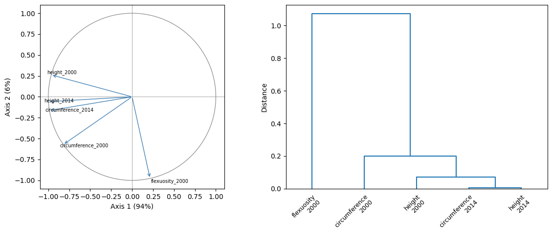
The factor-analytic can be read as a principal component analysis. Let us scale the genetic covariance to genetic correlation, interpret \(\mathbf{\Lambda_a}\) as a raw amount of \(\mathbf{\Sigma_a}\) explained by each axis, and study the structure of the genetic component of the traits in their correlative space.
# FA decomposition of the genetic covariance
S  = model.random[0].variance["sigma"]
fa = model.random[0].variance["metadata"]["fa"]
Q, Lam, Psi = fa["Q"], fa["Lambda"], fa["Psi"]
Gamma = Q * np.sqrt(Lam)

# correlation + clustering
Dn   = np.diag(1.0 / np.sqrt(np.diag(S)))
cor  = Dn @ S @ Dn
dist = 1.0 - cor
np.fill_diagonal(dist, 0.0)
dist = (dist + dist.T) * 0.5
Z = linkage(squareform(dist, checks=False), method="average")

# correlation circle
PC   = Dn @ Gamma
expl = Lam / np.trace(S)

# two aligned panels
fig, (ax1, ax2) = plt.subplots(1, 2, figsize=(12, 5))

ax1.add_patch(plt.Circle((0, 0), 1, fill=False, color="grey", lw=0.8))
ax1.axhline(0, color="grey", lw=0.5); ax1.axvline(0, color="grey", lw=0.5)
for i, name in enumerate(responses):
    ax1.annotate("", xy=(PC[i, 0], PC[i, 1]), xytext=(0, 0),
                 arrowprops=dict(arrowstyle="->", color="steelblue"))
    ax1.text(PC[i, 0] * 1.05, PC[i, 1] * 1.05, name, fontsize=7)
ax1.set_xlim(-1.1, 1.1); ax1.set_ylim(-1.1, 1.1); ax1.set_aspect("equal")
ax1.set_xlabel(f"Axis 1 ({100 * expl[0]:.0f}%)")
ax1.set_ylabel(f"Axis 2 ({100 * expl[1]:.0f}%)")

labels = [r.replace("_", "\n") for r in responses]
dendrogram(Z, labels=labels, ax=ax2, color_threshold=0)
ax2.set_ylabel("Distance")
ax2.tick_params(axis="x", labelsize= 9)
plt.setp(ax2.get_xticklabels(), rotation=45, ha="right", rotation_mode="anchor")

fig.tight_layout()
plt.show()
This yields a correlation circle allowing direct interpretation of the factorial axes, and a dendrogram clustering the responses with regards to the random effect.