Prediction

After fitting, pyreml can predict random effects at levels of unit that were not observed in the training data, for instance spatial interpolation or genomic prediction. This is available for effects whose right-hand factor relates the levels to one another:

right_hand	Prediction input over all levels (train + new)
str	A known covariance, through covariance.
dist	A known distance, through distance.
eucl / ar_iso / ar_ani	The coordinate tuples, through matrix_index.

For the coordinate kernels the coordinates are the level labels, so they are carried by matrix_index itself; for str and dist the matrix is supplied separately and matrix_index only orders its rows and columns.

Residuals can never be predicted, even when using a covariance structure or kernel. Consider including such structure with an extra random effect instead.

Prediction on-the-fly

The random effects can be directly obtained from Henderson’s equations with the new levels included as dummy individuals: carrying no observation, they are tied to the observed levels solely through their correlation to the observed ones expressed in \(\mathbf{K_a}\).

For the ar_iso and ar_ani, the whole grid is always predicted on-the-fly.

Prediction error variance

All the random effects \(\hat{\mathbf{u}}\) included in the HMME come with a Prediction Error Variance (PEV). The PEV and their covariance \(\mathbf{P}\) are computed all together as:

\[ \mathbf{P} = \mathbf{G} - \mathbf{G}\mathbf{Z}^\top\mathbf{V}^{-1}\mathbf{Z}\mathbf{G} + \mathbf{G}\mathbf{Z}^\top\mathbf{V}^{-1}\mathbf{X} (\mathbf{X}^\top\mathbf{V}^{-1}\mathbf{X})^{-1} \mathbf{X}^\top\mathbf{V}^{-1}\mathbf{Z}\mathbf{G}. \]

The PEV matrix for each random effect \(\mathbf{P_a}\) is then exposed as model.random[i].PEV.

Kriging

Solving the HMME requires the inversion of \(\mathbf{G}\), hence implicitely \(\mathbf{K_a}\), which can bottleneck when the number of levels to predict upscales.

For this reason, pyreml provides a kriging approach that consists in the sole inversion of the \(\mathbf{K}_{\text{train}}\), the submatrix of \(\mathbf{K_a}\) that only encompasses the levels included in the training set (i.e. the observed levels):

\[ \hat{\mathbf{a}}_{\text{pred}} = \mathbf{K}_{\text{pred}}\,\mathbf{K}_{\text{train}}^{-1}\, \hat{\mathbf{a}}_{\text{train}}, \]

with \(\hat{\mathbf{a}}_{\text{pred}}\) the pure prediction of unobserved levels, \(\hat{\mathbf{a}}_{\text{train}}\) the prediction of the observed levels (usually predicted at the HMME step), and \(\mathbf{K}_{\text{pred}}\) the covariance between the observed and non-observed levels.

• with str, \(\mathbf{K_a}\) is directly read from the supplied covariance structure;

preds = model.random[0].predict(
    matrix_index = full_index,   # all levels: train + new
    covariance   = K_full,
)

• with dist it is rebuilt from the supplied distance \(\mathbf{D}\) with the estimated decay \(\hat{\rho}\): \((\mathbf{K_a})_{ij} = \exp(-\hat{\rho}\, (\mathbf{D})_{ij})\);

preds = model.random[0].predict(
    matrix_index = full_index,   # all levels: train + new
    distance = D_full,
)

• with the coordinate kernels eucl, ar_iso and ar_ani, it is rebuilt from the coordinate tuples with the estimated rate(s), reusing the same Euclidean or autoregressive decay as in the fit.

preds = model.random[0].predict(
    matrix_index = full_index,   # all levels: train + new
)

matrix_index lists all levels, training and new; predict returns a long-format DataFrame with one row per (unit, response, component). When unit is a list of coordinate columns, those columns label the rows in place of a single unit.

Illustration

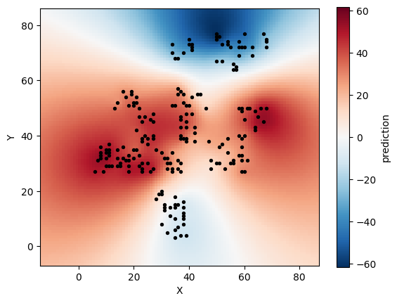
Let’s realize the spatial analysis of the larix illustrative dataset using the kriging prediction module.

import numpy as np
import matplotlib.pyplot as plt
from pyreml import MixedModel, Random, larix as df

# prepare data
df = df[df["year"] == 2000].copy()

# fit the model: coordinates are read directly from `unit`
mod = MixedModel.from_dataframe(
    data=df,
    response="height",
    fixed="1",
    random=Random(
        unit=["X", "Y"],
        right_hand="eucl",
    ),
).fit()

# build the prediction grid
coords = df[["X", "Y"]].to_numpy()

gx = np.arange(
    coords[:, 0].min() - 20,
    coords[:, 0].max() + 20,
)

gy = np.arange(
    coords[:, 1].min() - 10,
    coords[:, 1].max() + 10,
)

GX, GY = np.meshgrid(gx, gy)
grid = np.column_stack([GX.ravel(), GY.ravel()])

# coordinate tuples used as matrix indices
train_coords = [tuple(c) for c in coords]
grid_coords = [tuple(c) for c in grid]

# fitted BLUPs at the observed coordinates
train_blup = {
    coord: prediction
    for coord, prediction in zip(
        train_coords,
        mod.random[0].table["prediction"],
    )
}

# predict only genuinely new coordinates
new_coords = [
    coord
    for coord in grid_coords
    if coord not in train_blup
]

prediction_df = mod.random[0].predict(
    matrix_index=train_coords + new_coords,
)

# predicted values indexed by coordinate
predicted_blup = {
    (row["X"], row["Y"]): row["prediction"]
    for _, row in prediction_df.iterrows()
}

# observed cells use their fitted BLUP;
# unobserved cells use the kriging prediction
surface = np.array(
    [
        train_blup.get(coord, predicted_blup.get(coord))
        for coord in grid_coords
    ],
    dtype=float,
).reshape(GX.shape)

# plot the results
m = np.nanmax(np.abs(surface))

plt.imshow(
    surface,
    origin="lower",
    extent=[gx.min(), gx.max(), gy.min(), gy.max()],
    aspect="equal",
    cmap="RdBu_r",
    vmin=-m,
    vmax=m,
)

plt.colorbar(label="prediction")
plt.scatter(df["X"], df["Y"], c="black", s=8)
plt.xlabel("X")
plt.ylabel("Y")
plt.show()         

This models the spatial effect throughout the whole experimental design: