Training models
pyreml fits linear mixed models by direct differentiation of the Restricted Maximum Likelihood (REML) using PyTorch for variance parameter estimation. It benefits from PyTorch parallelization and GPU acceleration.
Fitting process
The fit method
Once a pyreml model is specified, it can be trained with the .fit() method.
model.fit()This runs the full pipeline, calling this series of methods:
.OLS(), Ordinary least squares (OLS) initialization of \(\mathbf{\beta}\),.REML(), REML estimation of the variance components,.HMME(), Henderson’s mixed model equations (HMME) for the random-effect predictions.
REML and HMME are engaged whenever the model carries random effects, a residual variance structure, or several responses; otherwise the fitting process stops at the OLS step.
Numerical resolution
The fit method takes a dtype argument:
"mixed"(default): OLS and a first REML pass run infloat32to approach the optimum cheaply, then a second REML pass and HMME run infloat64to refine the estimate and produce reliable outputs."double": all three steps (OLS, REML, HMME) run infloat64(\(=\)torch.double). This option is intended for GPUs optimized forfloat64where thefloat32warm-up is not useful."float": all three steps run infloat32. Fastest, but all outputs are single-precision and in some cases the REML solver can go off-track badly.
OLS
The fixed effects are first estimated by ordinary least squares,
\[ \hat{\mathbf{\beta}}_{\text{OLS}} = (\mathbf{X}^\top\mathbf{X})^{-1}\mathbf{X}^\top\mathbf{y}, \]
implying \(\mathbf{X}\) to be full-rank. If the model carries no random effect, an iid residual and a single response, then the OLS solution is already the answer and training stops here. Otherwise the OLS estimate initializes \(\mathbf{\beta}\) before REML. This initialization is always performed by .fit() and is strongly recommended for lower level uses of pyreml.
REML
REML loss
The per-effect blocks \(\mathbf{G_a} = \mathbf{\Sigma_a} \otimes \mathbf{K_a}\) (see Variance structures) are assembled into the full random-effect covariance by a direct sum over effects:
\[ \mathbf{G} = \bigoplus_\mathbf{a} \mathbf{G_a}, \]
and the marginal covariance of the observations follows as:
\[ \mathbf{V} = \mathbf{Z}\mathbf{G}\mathbf{Z}^\top + \mathbf{R}. \]
Because observations may be missing in unbalanced designs, \(\mathbf{\Sigma_R} \otimes \mathbf{K_R}\) is assembled over all original rows and then restricted to the observed entries through a residual “incidence” \(\mathbf{W}\) such as: \(\mathbf{R} = \mathbf{W}\left(\mathbf{\Sigma_R} \otimes \mathbf{K_R}\right)\mathbf{W}^\top\).
The variance parameters and \(\mathbf{\beta}\) are estimated by direct gradient descent of the negative log-likelihood (Simchoni & Rosset, 2023), restricted (REML) so as to yield unbiased estimates of the variance parameters (Harville, 1977; Patterson & Thompson, 1971):
\[ -2\ell_{\text{REML}} = \log\lvert\mathbf{V}\rvert + \mathbf{r}^\top\mathbf{V}^{-1}\mathbf{r} + \log\lvert\mathbf{X}^\top\mathbf{V}^{-1}\mathbf{X}\rvert + (n - p) \log(2\pi), \]
with \(\mathbf{r} = \mathbf{y}-\mathbf{X}\mathbf{\beta}\).
Optimization
The objective is optimized with L-BFGS (Liu & Nocedal, 1989) under a strong-Wolfe line search, with Adam (Kingma & Ba, 2017) as a fallback for steps the line search cannot complete. The variance parameters and \(\mathbf{\beta}\) are optimized jointly.
SMW
The REML computation uses the Sherman–Morrison–Woodbury identity (SMW) (Woodbury, 1950) which can have an important impact on the performance of the models depending on their specification.
Interest of SMW for REML
The use of SMW aims at avoiding forming and inverting \(\mathbf{V}\) directly:
\[ \begin{align} \mathbf{V}^{-1} &= \left(\mathbf{Z}\mathbf{G}\mathbf{Z}^{\top} + \mathbf{R}\right)^{-1} \\ &= \mathbf{R}^{-1} - \mathbf{R}^{-1}\mathbf{Z} \mathbf{C}^{-1} \mathbf{Z}^{\top}\mathbf{R}^{-1}, \end{align} \]
with the capacitance matrix \(\mathbf{C}\):
\[ \mathbf{C} = \mathbf{Z}^{\top}\mathbf{R}^{-1}\mathbf{Z} + \mathbf{G}^{-1}. \]
The associated determinant lemma gives the REML log-determinant without forming \(\mathbf{V}\) either:
\[ \log |\mathbf{V}| = \log |\mathbf{R}| + \log |\mathbf{G}| + \log |\mathbf{C}|. \]
Therefore, the problem transposes from inverting \(\mathbf{V}\) to inverting \(\mathbf{C}\), \(\mathbf{G}\) and \(\mathbf{R}\).
Using the properties of direct sum and Kronecker product:
\[ \mathbf{G}^{-1} = \bigoplus_\mathbf{a} (\mathbf{\Sigma_a}^{-1} \otimes \mathbf{K_a}^{-1}). \]
For the residual (see this section):
\[ \mathbf{R}^{-1} = \mathbf{W}\left(\mathbf{\Sigma_R}^{-1} \otimes \mathbf{K_R}^{-1}\right)\mathbf{W}^\top, \]
which only stands under some conditions, including:
- if \(\mathbf{W} = \mathbf{I}\);
- or if both \(\mathbf{\Sigma_R}\) and \(\mathbf{K_R}\) are diagonal, as \(\mathbf{W}\) is a mere row-column selector.
Most left-hand and right-hand term inverses can be broken down even further, avoiding expensive computations for \(\mathbf{G}^{-1}\) and \(\mathbf{R}^{-1}\). The SMW path trades the complexity of inverting a dense \(\mathbf{V}_{n \times n}\) for inverting a dense \(\mathbf{C}_{q \times q}\) at each step.
Implementation of SMW
SMW is usually more efficient when \(q < n\), with \(q\) the number of columns of \(\mathbf{Z}\) (the total dimension of \(\mathbf{u}\)) and \(n\) the number of stacked observations (i.e. \(\mathbf{Z}\) is narrower than tall). Indeed, inverting the \(q \times q\) matrix \(\mathbf{C}\) is cheaper than inverting the \(n \times n\) matrix \(\mathbf{V}\) only when \(q < n\).
pyreml mostly conforms to this “dimensional rule”, selecting SMW=True when \(q < n\), SMW=False otherwise.
However:
- using the high-level
from_dataframeconstructor, if the user forcesSMW=TrueorFalsethen their decision takes precedence over any other rule. - using the high-level
from_dataframeconstructor, if all of the following conditions are met then SMW is switched off regardless of the dimensional rule:- \(\mathbf{W} \neq \mathbf{I}\), which can arise for instance with several unbalanced options, or when using autoregressive structures.
- the residual covariance \(\mathbf{R}\) is not designed as a diagonal matrix.
Indeed, in this situation \(\mathbf{R}^{-1} \neq \mathbf{W}\left(\mathbf{\Sigma_R}^{-1} \otimes \mathbf{K_R}^{-1}\right)\mathbf{W}^\top\) and inverting the \(n \times n\) matrix \(\mathbf{R}\) is just as expensive as inverting \(\mathbf{V}\).
- with the low-level constructor:
- if
varmeth_invonly is provided, SMW is forced on; - if
varmethonly is provided, SMW is forced off; - if both methods are available, the dimensional rule applies.
- if
Structured forward
Consider a random regression with three levels and four observations, an intercept and a covariate \(x\) being carried on each level:
\[ \newcommand{\z}{{\color{lightgray}0}} \mathbf{Z_a} = \begin{pmatrix} 1 & \z & \z & x_1 & \z & \z\\ 1 & \z & \z & x_2 & \z & \z\\ \z & 1 & \z & \z & x_3 & \z\\ \z & \z & 1 & \z & \z & x_4 \end{pmatrix}. \]
\(\mathbf{Z_a}\) can be entirely described by the pair \((\mathbf{F_a}, s)\), defined as the values each observation carries and the level it loads them on:
\[ \mathbf{F_a} = \begin{pmatrix} 1 & x_1\\ 1 & x_2\\ 1 & x_3\\ 1 & x_4 \end{pmatrix}, \qquad s = (1, 1, 2, 3). \]
Row \(i\) of \(\mathbf{F_a}\) is written \(\mathbf{f}_i\), and \(s(i)\) is the level loaded by observation \(i\). Over several responses, \(\mathbf{F_a}\) is block-diagonal: each row carries the values of its own response, matching the response blocks of \(\mathbf{\Sigma_a}\).
Assembling \(\mathbf{V_a} = \mathbf{Z_a}\mathbf{G_a}\mathbf{Z_a}^\top\) directly forms the Kronecker block \(\mathbf{G_a} = \mathbf{\Sigma_a} \otimes \mathbf{K_a}\), then multiplies through every column of \(\mathbf{Z_a}\). Yet each row of \(\mathbf{Z_a}\) being confined to a single level, entry \((i,j)\) of that product reduces to the covariance between the values carried by observations \(i\) and \(j\), scaled by the kernel entry between the levels they load:
\[ [\mathbf{V_a}]_{ij} = \mathbf{f}_i^\top\,\mathbf{\Sigma_a}\,\mathbf{f}_j\, [\mathbf{K_a}]_{s(i)\,s(j)}. \]
The right-hand factor collects into \(\mathbf{K_a}\) read at the observed level pairs:
\[ \left[\mathbf{K_a}^{\text{obs}}\right]_{ij} = \left[\mathbf{K_a}\right]_{s(i)\,s(j)}, \qquad \mathbf{K_a}^{\text{obs}} = \begin{pmatrix} K_{11} & K_{11} & K_{12} & K_{13}\\ K_{11} & K_{11} & K_{12} & K_{13}\\ K_{21} & K_{21} & K_{22} & K_{23}\\ K_{31} & K_{31} & K_{32} & K_{33} \end{pmatrix}, \]
so that the whole contribution is written as a Hadamard (elementwise) product \(\odot\):
\[ \mathbf{V_a} = \left(\mathbf{F_a}\,\mathbf{\Sigma_a}\,\mathbf{F_a}^\top\right) \odot \mathbf{K_a}^{\text{obs}}. \]
Neither \(\mathbf{G_a}\) nor \(\mathbf{Z_a}\mathbf{G_a}\mathbf{Z_a}^\top\) is ever formed, sparing both the memory and the time they would cost. This was exemplified with random regression, but holds for any effect built by from_dataframe. The full covariance follows as \(\mathbf{V} = \sum_\mathbf{a} \mathbf{V_a}\), residual included.
On the SMW path, a second structured forward optimization is applied to prevent the formation of \(\mathbf{R}^{-1}\) and of the Kronecker block \(\mathbf{\Sigma_R}^{-1} \otimes \mathbf{K_R}^{-1}\) it is read from. Any \(\mathbf{Z}\), \(\mathbf{X}\) or \(\mathbf{r}\) column can be reshaped as a matrix \(\mathbf{U}\) over the level \(\times\) response grid:
\[ \mathbf{R}^{-1}\operatorname{vec}(\mathbf{U}) = \operatorname{vec}\left(\mathbf{K_R}^{-1}\,\mathbf{U}\,\mathbf{\Sigma_R}^{-1}\right). \]
The levels are contracted along the rows, the responses along the columns, and the result is flattened back. Two small products replace one large inverse, which is never formed. Unbalanced designs leave part of the grid empty, which is what the residual incidence \(\mathbf{W}\) encodes. Operands are therefore lifted onto the complete grid, contracted, and read back at the observed cells afterwards.
The structured forward path is switched off when:
- using the
from_dataframehigh level builder, the user forcesstructured_forward = False; - always when using the low level builder.
Analytical backward
The REML gradient with respect to any variance parameter \(\theta\) has a closed form: \[ \frac{\partial(-2\ell_{\text{REML}})}{\partial\theta} = \operatorname{tr}\!\left(\mathbf{A}\,\frac{\partial\mathbf{V}}{\partial\theta}\right), \] \[ \mathbf{A} = \mathbf{V}^{-1} - \mathbf{V}^{-1}\mathbf{r}\mathbf{r}^\top\mathbf{V}^{-1} - \mathbf{V}^{-1}\mathbf{X} \left(\mathbf{X}^\top\mathbf{V}^{-1}\mathbf{X}\right)^{-1} \mathbf{X}^\top\mathbf{V}^{-1}, \]
with \(\partial(-2\ell_{\text{REML}})/\partial\mathbf{\beta} = -2\,\mathbf{X}^\top\mathbf{V}^{-1}\mathbf{r}\). As \(\mathbf{V} = \sum_\mathbf{a}\mathbf{V_a}\), for a given random effect (or the residual), the trace permutes into:
\[ \frac{\partial(-2\ell_{\text{REML}})}{\partial\theta_\mathbf{a}} = \operatorname{tr}\!\left(\mathbf{Z_a}^\top\mathbf{A}\,\mathbf{Z_a}\; \frac{\partial\mathbf{G_a}}{\partial\theta_\mathbf{a}}\right). \]
\(\mathbf{A}\) is therefore evaluated once at the current point and shared by every variance parameter. Reusing the decomposition of structured forward, where \(\mathbf{Z_a}\) is replaced by \((\mathbf{F_a}, s)\) and \(\mathbf{G_a}\) by \(\mathbf{\Sigma_a}\) and \(\mathbf{K_a}\), the trace contracts onto each variance matrix:
\[ \frac{\partial(-2\ell_{\text{REML}})}{\partial\mathbf{\Sigma_a}} = \mathbf{F_a}^\top\left(\mathbf{A} \odot \mathbf{K_a}^{\text{obs}}\right)\mathbf{F_a}, \qquad \left[\frac{\partial(-2\ell_{\text{REML}})}{\partial\mathbf{K_a}}\right]_{st} = \sum_{\substack{i\,:\,s(i)=s \\ j\,:\,s(j)=t}} \left[\mathbf{A} \odot \mathbf{F_a}\mathbf{\Sigma_a}\mathbf{F_a}^\top\right]_{ij}. \]
On the SMW path, \(\mathbf{V}\) is never formed, so neither is \(\mathbf{A}\). The trace is then read in the level space, from \(\mathbf{Z}^\top\mathbf{A}\mathbf{Z}\) directly:
\[ \mathbf{Z}^\top\mathbf{A}\mathbf{Z} = \mathbf{Z}^\top\mathbf{V}^{-1}\mathbf{Z} - \left(\mathbf{Z}^\top\mathbf{V}^{-1}\mathbf{r}\right)\left(\mathbf{Z}^\top\mathbf{V}^{-1}\mathbf{r}\right)^\top - \left(\mathbf{Z}^\top\mathbf{V}^{-1}\mathbf{X}\right)\left(\mathbf{X}^\top\mathbf{V}^{-1}\mathbf{X}\right)^{-1}\left(\mathbf{Z}^\top\mathbf{V}^{-1}\mathbf{X}\right)^\top \] which uses 3 quantities the SMW projection already delivers through \(\mathbf{C}\):
\[ \mathbf{Z}^\top\mathbf{V}^{-1}\mathbf{M} = \mathbf{Z}^\top\mathbf{R}^{-1}\mathbf{M} - \left(\mathbf{Z}^\top\mathbf{R}^{-1}\mathbf{Z}\right)\mathbf{C}^{-1}\left(\mathbf{Z}^\top\mathbf{R}^{-1}\mathbf{M}\right), \qquad \mathbf{M} \in \{\mathbf{Z}, \mathbf{r}, \mathbf{X}\} \]
PyTorch autograd is therefore disabled through the assembly and factorisation of \(\mathbf{V}\) (\(\mathbf{C}\) on the SMW path). Automatic differentiation is only left with the last step, from each variance matrix to its own parameterization, and never traverses the Kronecker products.
The analytical backward path is switched off when:
- using the
from_dataframehigh level builder, the user forcesanalytic_backward = False; - always when using the low level builder.
Convergence criterion
Convergence is declared when two successive evaluations of \(-2\ell_{\text{REML}}\) agree to within a tolerance \(\tau\), the smallest difference in likelihood that remains meaningful given both the numerical resolution of the evaluation and the scale on which likelihoods are compared:
\[ \tau = \min\left( \tau_{\max},\; \lvert -2\ell_{\text{REML}} \rvert \cdot 10^{-\delta_\text{tot}} \right), \qquad \delta_\text{tot} = \min\left(\delta_{\max},\; \delta_e - \left(\delta_{c} + \delta_{r} + \delta_{\kappa}\right) \right). \]
The restricted likelihood grows with the number of observations: the same dataset measured twice as often returns a value roughly twice as large. A fixed absolute threshold would therefore demand ever more significant digits as the dataset grows, and eventually more than the computer can hold. Counting significant digits keeps that demand constant. The budget starts from the machine epsilon \(e\) of the working precision \((\delta_e = -\log_{10}(e) \approx
15.65\) in float64, \(\approx 6.92\) in float32) and is capped by the conservative ceiling \(\delta_{\max} = 10\). The three positive corrections count digits that are certain to be noise: \(\delta_c\) carries the cumulated uncertainty of the elementary components the likelihood is summed from, while \(\delta_r\) and \(\delta_\kappa\) address the inversion of the variance \(\mathbf{V}\) (or the capacitance \(\mathbf{C}\) on the SMW path): \(\delta_r\) as a random walk over the many operations of the factorisation, \(\delta_\kappa\) as the information lost to the conditioning of the matrix. They are amplification factors that compound, hence the sum. Each is a conservative proxy, and \(\delta_\text{tot}\) an estimate of the surviving resolution: no REML step is spent refining a decimal that carries no information.
The digit budget is relative, but what makes a likelihood difference meaningful is absolute: two models separated by \(\Delta\)AIC \(= 2\) are considered distinguishable. The ceiling \(\tau_{\max} = 0.02\), one hundredth of that scale, keeps the tolerance well below it. When the digit budget alone would push \(\tau\) past \(\tau_{\max}\), the noise floor of the evaluation has reached the scale at which models are told apart: the fit is reported as degenerate, the tolerance is clamped to \(\tau_{\max}\), and convergence is denied.
The tolerance \(\tau\) and the digit budget \(\delta_\text{tot}\), \(\delta_e\), \(\delta_{c}\), \(\delta_{r}\) and \(\delta_{\kappa}\) are returned in the logs, where degenerate cases can be diagnosed.
HMME
With the estimated variance components treated as known, the fixed and random effects are obtained jointly from Henderson’s mixed model equations (Henderson, 1975):
\[ \begin{bmatrix} \mathbf{X}^\top\mathbf{R}^{-1}\mathbf{X} & \mathbf{X}^\top\mathbf{R}^{-1}\mathbf{Z} \\ \mathbf{Z}^\top\mathbf{R}^{-1}\mathbf{X} & \mathbf{Z}^\top\mathbf{R}^{-1}\mathbf{Z}+\mathbf{G}^{-1} \end{bmatrix} \begin{bmatrix} \hat{\mathbf{\beta}} \\ \hat{\mathbf{u}} \end{bmatrix} = \begin{bmatrix} \mathbf{X}^\top\mathbf{R}^{-1}\mathbf{y} \\ \mathbf{Z}^\top\mathbf{R}^{-1}\mathbf{y} \end{bmatrix}. \]
Their solution gives the best linear unbiased estimator (BLUE) of \(\mathbf{\beta}\) and the best linear unbiased predictor (BLUP) of \(\mathbf{u}\), in a single solve.
The same system also yields the error variances of the estimates and predictions. See Prediction for the prediction error variance of \(\hat{\mathbf{u}}\).
Akaike information criterion
Once the model is fitted, the Akaike information criterion (AIC) is computed in two different ways depending on whether it was performed by OLS or HMME/REML. The AIC is available as attribute AIC and the AIC method is recorded as AIC_meth.
These two AICs should not be compared with each other. AIC computed post-OLS is designed for the exploration of fixed effects with no variance structure, and AIC computed post REML/HMME is designed for the investigation of the variance structure with a fixed \(\mathbf{X}\) (i.e. a fixed formula in the model specification).
AIC post OLS is computed using the likelihood, from the unbiased residual variance \(\sigma^2_R\):
\[ -2\ell_{\text{ML}} = n \log\left( \frac{n-p}{n} \sigma^2_R \right) + n + n \log(2\pi) \]
and AIC post REML/HMME is computed using the restricted likelihood (\(-2\ell_{\text{REML}}\)).
In both cases, AIC is obtained by the addition of twice the total number of parameters (\(\beta\), and all independent variance parameters).
Monitoring
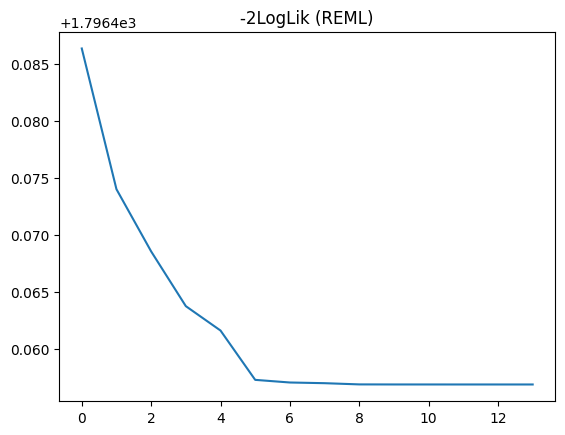
The fit can be followed through the REML objective recorded at each iteration and a convergence flag, both exposed on the model.
| Accessor | Content |
|---|---|
model.opti_REML.loss |
The REML objective at each iteration. |
model.opti_REML.converged |
Whether the convergence criterion was met. |
model.opti_REML.duration |
Wall-clock time of the REML fit, in seconds. |
L-BFGS drives the optimization and Adam steps in only to recover iterations the line search cannot complete; occasional Adam steps near a difficult region of the objective are expected.
As an illustration, the last iterations of an example model REML convergence:
import matplotlib.pyplot as plt
plt.plot(model.opti_REML.loss)
plt.title("-2LogLik (REML)")
plt.show()