Random regression and factors
Each random effect of a pyreml model takes a formula specification, that is reminescent of the (1 + x | unit) idiom in lme4. This formula should be comprehensive for patsy. Each column read from this formula (intercept, regressor, modalities of factors, and interactions) becomes a component of the effect that varies from one unit to the next.
The left-hand factor \(\mathbf{\Sigma_a}\) models the covariance between these components (see variance structures).
Random regression
A formula including a regression, such as "1 + x", gives each unit its own random intercept and its own random slope.
Random(
    unit       = "patient",
    formula    = "1 + x",
    left_hand  = "full",
    right_hand = "iid",
)
Developing this example:
\[ y_{ij} = (\beta_0 + a_{0i}) + (\beta_{1} + a_{1i})\, x_{j} + r_{ij}, \qquad \begin{bmatrix} \mathbf{a_{0}} \\ \mathbf{a_{1}} \end{bmatrix} \sim \mathcal{N}(\mathbf{0}, \mathbf{\Sigma_a} \otimes \mathbf{I}), \]
Where \(j\) is the index for the longitudinal variable (for instance, the time or a dose of treatment) and \(i\) is the index for the random effect unit (for instance, an individual).
Random factors
A formula can also carry a factor, or the interaction between factors, so that the effect of each of its modalities is random across units. For instance:
Random(
    unit       = "patient",
    formula    = "0 + C(treatment)",
    left_hand  = "full",
    right_hand = "iid",
)
Each treatment now contributes one random component per patient, and the left-hand factor \(\mathbf{\Sigma_a}\) (across modalities of treatments) captures how those treatment effects covary.
Illustration
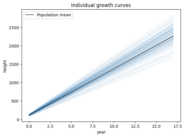
Let’s realize a random regression on the larix illustrative dataset, modeling individual tree growth along years.
import numpy as np
import matplotlib.pyplot as plt
from pyreml import (
    MixedModel,
    Random,
    Residual,
    A_pedigree,
    prepare_pedigree,
    larix as df
)

# scale years
df = df.copy()
df["year"] = df["year"] - df["year"].min()

mod = MixedModel.from_dataframe(
    data     = df,
    response = "height",
    fixed    = "1 + year",
    random   = [
        Random(
            unit         = "ID",
            formula      = "1 + year",
            left_hand    = "full",
            right_hand   = "iid",
        ),
    ],
    residual = Residual(
        left_hand = "iid",
        right_hand = "het",
        het_formula = "C(year)"
    )
).fit()

# fixed effects
b = mod.estimates.set_index("term")["estimate"]
b0, b1 = b["Intercept"], b["year"]

# individual effects
re = mod.random[0].table.pivot_table(
    index   = "unit",
    columns = "component",
    values  = "prediction"
)

yr  = np.linspace(df["year"].min(), df["year"].max(), 100)

fig, ax = plt.subplots(figsize=(7, 5))

# individual curves
for _, row in re.iterrows():
    a0, a1 = row["Intercept"], row["year"]
    ax.plot(
        yr,
        (b0 + a0) + (b1 + a1) * yr,
        color = "#4B8BBE",
        lw    = 0.6,
        alpha = 0.15
    )

# population curve
ax.plot(
    yr,
    b0 + b1 * yr,
    color = "black",
    lw    = 1,
    label = "Population mean"
)
plt.title("Individual growth curves")
ax.set_xlabel("year"); ax.set_ylabel("height")
ax.legend()
plt.show()

# correlations
def cov2cor(cov):
    std = np.sqrt(np.diag(cov))
    print(cov / np.outer(std, std))

cov2cor(mod.random[0].variance["sigma"])
Each individual ends up with specific random parameters for a regression. Note that the residual variance was choose as year-specific, year being treated as a factor (C(year)) in the heteroscedasticity specification.